
What is Feature Engineering and why do we need it?
Raw spatial data like the one we downloaded from OSM is often not directly useful for analysis or modeling. This is where Feature Engineering comes in. Feature Engineering is the process of transforming this raw data into meaningful variables (features) that machine learning models can use. This process may involve cleaning data, transforming values, or creating new variables that better capture relevant patterns.
Models learn from the features you give them. Well-designed features make patterns easier to detect, which can improve accuracy and help the model generalize better to new data. In many cases, good feature engineering has a bigger impact than choosing a more complex model.
In this notebook, we will be using our raw OSM data to detect all intersections inside our bounding box as well as related statistics. These intersections will then serve as a new feature for further analysis.
Why Analyse Intersections?
Intersections act as the critical nodes of a city’s infrastructure, defining traffic flow, safety, and neighborhood character. By analysing their geometry and connectivity, we can distinguish between areas optimized for pedestrians versus those designed for heavy vehicle traffic. Irregular or highly skewed intersections often correlate with increased accident risks or inefficient traffic flows. Quantifying these characteristics allows us to move beyond simple mapping and better understand how a city functions.
Thus, intersections provide a meaningful and informative feature for further analysis.
Imports and Configuration
First, we will import all necessary libaries and custom functions.
import sys
from dataclasses import asdict
from pathlib import Path

import folium
import geopandas as gpd
import iplotx as ipx
import matplotlib.pyplot as plt
import pandas as pd
import pyproj
from folium import Element
from shapely import wkb

# ruff: noqa: T201

# Importing custom functions
sys.path.append(str(Path("..").resolve()))
from src.geoai.cookbook_functions import (
    IntersectionAnalyzer,
    OSMLoader,
    OSMProcessor,
    get_base_map,
    run_streaming_process_in_memory,
)

# Configuration
CITY_NAME = "Vienna"
BBOX = "16.335005,48.187854,16.400923,48.209995"
DATA_DIR = "./osm_data"
OUTPUT_DIR = "./output"

# Computing the center of the bounding box
min_lon, min_lat, max_lon, max_lat = map(float, BBOX.split(","))
bounds = [[min_lat, min_lon], [max_lat, max_lon]]
center_lat = (min_lat + max_lat) / 2
center_lon = (min_lon + max_lon) / 2

# check if file exists and download if not
xml_file_path = (Path(DATA_DIR) / f"{CITY_NAME}.xml").resolve()

loader = OSMLoader(DATA_DIR)

if not xml_file_path.exists():
    loader.download_within_bbox(BBOX, CITY_NAME)

nodes, ways, rels, walk, car = run_streaming_process_in_memory(xml_file_path)
Attempting download from: https://overpass-api.de/api/map?bbox=16.335005,48.187854,16.400923,48.209995
Download complete.
You can take a look at the file at: /builds/cookbooks/private/intersection-analysis-cookbook/notebooks/osm_data/Vienna.xml
Finding the Intersections
In the next step we compute all intersections inside our target area using a custom function. We can roughly break this process down into three distinct steps which will be explained now.
Parsing the file
First, we parse the XML file. Since OSM files can be massive, we cannot load everything into memory at once, or we might run out of RAM before we even start the analysis. Instead, we use a Streaming approach with a Two-Pass Strategy to be memory efficient.
We read the file twice to avoid saving unnecessary data:
Pass 1: We scan the file looking only for ways (lines). If a way is relevant (e.g., has a highway tag that is relevant for us like “primary road”), we note down the IDs of the nodes it uses.
Pass 2: We read the file again, this time looking for nodes (points). We only keep the nodes that were found to be relevant in the first pass and discard the rest immediately.
This allows us to process large areas using relatively little RAM. During this process, we also immediately separate the data into “walkable” paths and “drivable” roads to analyse them independently.
nodes, ways, rels, walk, car = run_streaming_process_in_memory(xml_file_path)

print(f"Loaded {len(nodes)} nodes and {len(ways)} ways.")
Loaded 30940 nodes and 10900 ways.
Processing the Networks
Raw OSM data often contains many small segments for a single street. To get accurate intersection counts, we need to consolidate these. We use a custom processor function to simplify the IDs and merge duplicate segments connecting the same points for both the walking and driving networks.
# Process Walk Network
p_walk = OSMProcessor("walk", nodes, ways, rels, walk)
p_walk.simplify_ids()
m_walk = p_walk.get_merged_segments()

# Process Car Network
p_car = OSMProcessor("car", nodes, ways, rels, car)
p_car.simplify_ids()
m_car = p_car.get_merged_segments()

print("Network processing complete.")
Network processing complete.
Computing the Intersections and Statistical Values
Now we build the network graph. If you look into the custom code for creating the network graph, you will see, that we create the network container using the Networkx library.
What is Networkx?
NetworkX is an open-source Python library for creating, analyzing, and visualising networks and graph structures. It provides tools for working with nodes and edges, making it useful for studying all types of networks, like the street network we are working with, and spatial connectivity.
With NetworkX, complex graph operations such as shortest path analysis, centrality measures, and network traversal can be performed directly in Python, making it one of the most widely used libraries for network analysis and graph-based workflows.
We can have a look at our street network by plotting it with the iplotx and matplotlib libaries.
# Set up the ouput directory
out_dir = Path(OUTPUT_DIR) / CITY_NAME
out_dir.mkdir(parents=True, exist_ok=True)

# Initialize the Analyser
analyzer = IntersectionAnalyzer(final_path=out_dir)

# Build the Graph
way_tags = analyzer.build_graph(nodes, ways, m_walk, m_car)

G = analyzer.graph

# Projecting to metric space
project = pyproj.Transformer.from_crs(
    "EPSG:4326", "EPSG:3857", always_xy=True
).transform

layout = {n: project(d["lon"], d["lat"]) for n, d in G.nodes(data=True)}

# Setting up the plot
fig, ax = plt.subplots(figsize=(14, 10))

# Setting up the network graph
ipx.network(
    G,
    layout,
    ax=ax,
    node_size=0,
    edge_linewidth=0.3,
    edge_color="black",
    alpha=0.6,
)

ax.set_aspect("equal", adjustable="box")
ax.axis("off")

plt.tight_layout()
plt.show()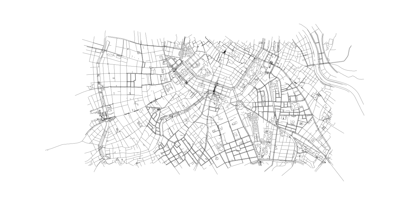
After building the network graph, we can finally identify all intersections in our network. We define intersections as nodes that have a minimum of three ways connected to it, and calculate some statistical values for each intersection.
Here is a quick overview over all columns of our output data we are generating in this step:
osm_id: This is the OSM intersection ID which is unique to each intersection.
i_tpe: This is the type of the intersection which tells us if it is used by pedestrians only (Path), cars only (Car) or both (Road).
num_ways: This tells us about the number of ways connected to the intersection, e.g. how many ways lead to it / away from it. It is at minimum 3 because of our definition of an intersection.
delta: This angle indicates the irregularity or “skewness” of the intersection, it tells us how much it deviates from a “perfect” intersection of its type (for a 3-way intersection that would be a Y-shaped intersection with each angle being exactly 120°).
delta_t: This value is similar to delta, but specifically for T-shaped intersections, e.g. an intersection connected to 3 ways at a right angle. For all intersections with more arms it is automatically set to 360 as those cannot be T-shaped.
geom: This variable saves the geometry of the intersection in WKB (Well-Known Binary) which is not human-readable.
We then convert the result into a GeoDataFrame so we can use it for the further processing and save the results to a CSV file which we can inspect.
What is a GeoDataFrame? What is GeoPandas?
A GeoDataFrame (GDF) is a central concept in GeoPandas. It is an extension of the pandas DataFrame that includes a geometry column for storing spatial objects such as points, lines, and polygons. GeoDataFrames combine geographic data with standard tabular data and support spatial operations such as projections, buffering, spatial joins, and distance calculations. Because they integrate spatial and attribute data in a single structure, GeoDataFrames are fundamental to efficient geospatial analysis and visualization workflows.
GeoPandas is an open-source Python library that makes working with geospatial data easier. It extends pandas with support for spatial data types and integrates with Shapely for geometric operations.
With GeoPandas, many spatial operations that would normally require a geospatial database such as PostgreSQL with the PostGIS extension (like mentioned in the Geospatial Databases cookbook!) can be performed directly in Python.
# Analyse Intersections (Calculate Metrics)
analyzer.analyze(way_tags, 3)

# Convert results to a GeoDataFrame
if analyzer.intersection_infos:
    # Convert list of dataclasses to DataFrame
    df_int = pd.DataFrame([asdict(i) for i in analyzer.intersection_infos])

    # Convert the 'geom' hex string back into Shapely Point objects.
    df_int["geometry"] = df_int["geom"].apply(lambda x: wkb.loads(bytes.fromhex(x)))

    # Create the GeoDataFrame using the new 'geometry' column
    intersections_gdf = gpd.GeoDataFrame(df_int, geometry="geometry", crs="EPSG:4326")

    # Save to CSV for inspection
    out_file = out_dir / "intersections.csv"
    df_int.drop(columns=["geometry"]).to_csv(out_file, index=False)

    print(f"\nSuccess! Found {len(intersections_gdf)} intersections.")
    print(f"You can find the CSV file here: {out_file}")
else:
    print("No intersections found.")
Success! Found 8518 intersections.
You can find the CSV file here: output/Vienna/intersections.csv
Finally, we can use Folium to take a look at the intersections we found. When you click on one of the intersections you can also see its statistical values.
# Setting up the map
m_final = get_base_map(center_lat, center_lon)

# Create a feature group for all intersection points
fg_pts = folium.FeatureGroup(name="Points", show=True)

for _, row in intersections_gdf.iterrows():
    # Color logic
    color = "blue"
    if row.get("i_tpe") == "Car":
        color = "crimson"
    elif row.get("i_tpe") == "Path":
        color = "green"

    # Popup
    popup_html = f"""
    <div style="font-family: sans-serif; font-size: 12px;">
        <b>ID:</b> {row.get("osm_id")}<br>
        <b>Type:</b> {row.get("i_tpe")}<br>
        <b>Arms:</b> {row.get("num_ways")}<br>
        <b>Delta:</b> {row.get("delta"):.2f}<br>
    </div>
    """

    folium.CircleMarker(
        [row.geometry.y, row.geometry.x],
        radius=1,
        color=color,
        fill=True,
        popup=folium.Popup(popup_html, max_width=200),
    ).add_to(fg_pts)

# Add the FeatureGroup to the map
fg_pts.add_to(m_final)

# Folium doesn't have a built-in categorical legend, so we define one using HTML.
legend_html = """
<div style="
    position: fixed;
    bottom: 50px; left: 50px; width: 160px; height: 110px;
    border:2px solid grey; z-index:9999; font-size:14px;
    background-color:white; opacity: 0.8;
    padding: 10px;
    border-radius: 5px;
    ">
    <b>Intersection Type</b><br>

    <span style="
        display:inline-block;
        width:10px;
        height:10px;
        background-color:green;
        border-radius:50%;
        margin-right:6px;
    "></span> Pedestrian Only<br>

    <span style="
        display:inline-block;
        width:10px;
        height:10px;
        background-color:blue;
        border-radius:50%;
        margin-right:6px;
    "></span> Mixed<br>

    <span style="
        display:inline-block;
        width:10px;
        height:10px;
        background-color:crimson;
        border-radius:50%;
        margin-right:6px;
    "></span> Car Only<br>
</div>
"""

# Add the legend to the map
m_final.get_root().html.add_child(Element(legend_html))

# Display the map
m_finalSummary
In this notebook you learned:
What Feature Engineering is and why it is important
What Networkx is and how to plot a network
What a GeoDataFrame is and why it is important
How to compute intersections in OSM data as a new feature